Hierarchical Timing Analysis: Pros, Cons, and a New Approach

To ensure that a digital semiconductor design works as planned, design teams use static timing analysis to determine if the clocks and signals are correctly timed. Currently, static timing analysis is performed flat or hierarchically, mostly depending on the size of the design. Flat analysis provides the most accurate results, as it is completely transparent down to the logic cells, but it requires more memory and a significant amount of time to run because every cell and every wire in the design is analyzed. It’s no wonder that, as design sizes continue to grow, designers are looking to hierarchical methodologies to help alleviate huge runtimes.

Using a hierarchical approach, a designer selects and times certain blocks of logic, generating results more quickly and with fewer memory resources. These blocks are then modeled as timing abstractions at the top level of the design to reduce the overall amount of detailed analysis in the final stages. This hierarchical approach minimizes the time to get results but with less accuracy. This paper covers the pros and cons of different hierarchical analysis approaches, and also provides some options for avoiding the tradeoffs inherent in this methodology to achieve efficient and accurate timing analysis.

Today, designs are so large, and design complexity is so high, that it’s common for a team of engineers to work together on a single chip using a hierarchical design methodology. Timing budgets are created throughout the design, typically at the pins of blocks, which enable team members to close timing on their blocks independent of top-level analysis. This methodology enables hierarchical analysis to be more practical, but still leaves the possibility that some critical timing issues can be missed, especially in paths that cross hierarchical boundaries.

The next two sections take a look at modeling used in hierarchical timing analysis. Modeling the timing of a hierarchical block can take one of several forms with each format having its pros and cons. The two most common are the Extracted Timing Model (ETM), which takes the form of a Liberty model (.lib), and the Interface Logic Model (ILM), which takes the form of a reduced netlist of interface logic and associated parasitic capacitance information.

Extracted Timing Model

As shown in Figure 1, ETMs use abstraction to minimize the amount of data while attempting to preserve accuracy. ETMs replace respective blocks in hierarchical timing analysis, which significantly speed-up analysis and reduce the memory footprint for the full-chip analysis. 

The fact that most ETMs have some deficiencies that hamper efficient and/or accurate hierarchical analysis should not be ignored because managing these limitations adds to runtime and solution complexity. ETM limitations and complexities include generation, validation, and merging of the ETM; signal integrity (SI) -aware ETMs; multi-mode, multi-corner (MMMC) ETM generation; multiple clocks on same pins/ports; advanced on-chip variation (AOCV) limitations; accuracy; multiple-master clock modeling for a generated clock; path exceptions modeling; waveform propagation-aware ETMs; and given scope. Let’s take a quick look at some of these items:

Model generation, validation, and merging

ETM generation and validation needs a special flow setup. In addition, ETMs that include multiple-constraint modes must be merged into a single ETM for usage at the top level of the chip.

SI-aware ETMs

Comprehension of SI in ETM generation is not very robust. Design teams typically adapt to the methodology by making interface logic SI clean before extracting ETMs. Generation of ETMs with SI significantly adds to the model generation runtime because in-context aggressor nets need to be accounted for. The generation of timing window information at the top level of the design is also necessary.

MMMC ETM generation

ETMs can be merged across the modes but not across the corners. MMMC analysis and variation requires extra allocation of time to extract ETMs that comprehensively cover all corners and modes.

Multiple clocks on same pins/ports

Application of multiple clocks on the same pins/ports is not allowed in certain timing-analysis tools. Design teams must take extra steps to provide an equivalent modeling for ETM generation.

AOCV limitations

AOCV-based ETM generation poses challenges for cases of multiple instantiated blocks, because the delays inside the ETMs are pre-derated based on the top-level context used during ETM characterization. These limitations are in addition to MMMC analysis, which imposes characterization per analysis view. For the same view, multiple characterizations for AOCV are required.

Accuracy

In some cases, interconnects at the ports must be abstracted, which can lead to accuracy loss. However, this loss might not be very significant.

Multiple-master clock modeling for a generated clock

The Liberty format is unable to specify the master clock of a generated clock. In the case of multiple masters, design teams must therefore provide external constraints to associate the generated clocks with the specific master clock, which can be cumbersome.

Path exceptions modeling

In certain situations, path exceptions must be re-coded for ETMs, e.g., when there are multiple output delays on a port and one of the output delays has a multi-cycle path (MCP) through one pin internal to the block. Unless one successfully preserves that internal pin (which increases the size of the model) or duplicates the ports for that MCP, design teams must create and manage exceptions to achieve the same timing result as flat analysis.

Waveform propagation-aware ETM

A missing comprehension of the waveform propagation effect inside ETMs leads to optimism and poses a challenge for lower geometries on its usage.

Given scope

ETMs are guaranteed to work accurately in a given context. Context means the conditions under which the design is analyzed. This can be physical context such as what surrounds the ETM in terms of other signals or it can mean electrical context such as power supply and voltage drop values seen by the ETM. Because many of these contexts are not known until near the end of the design cycle, they cannot be accurately taken into account during the ETM generation. Therefore, when the context changes, ETMs must be regenerated to be as accurate as possible.

Interface Logic Model

ILMs remove the register-to-register logic and preserve the rest of the interface logic in the model as shown in Figure 2. The components within an ILM include a netlist, parasitic loading, constraints, and aggressor information pertinent to the preserved logic inside the ILM. ILMs are highly accurate and can also speed up analysis considerably, while reducing the memory footprint.

Because ILMs preserve the interface logic exactly the same way as the original netlist, they can deliver exactly the same timing for interface paths as a flat analysis. Contextual impacts to the interface logic are observed by merging the ILM netlist, parasitic, and constraints into the chip-level components. ILM limitations include over-the-block routing, constraint mismatches, data management, arrival pessimism, latch-based designs, specific flows, and special stitching.

Over-the-block routing

If blocks are characterized without over-the-block routing in place, the timing could be optimistic since the SI impact of the over-the-block routes is not accounted for. This includes the cross coupling from over-the-block aggressor nets to victim nets within the block. Figure 3 illustrates this point.

Constraint mismatches

Additional bookkeeping is needed to preserve the context information. Mismatches in constraint are a significant headache for the designer and can be a major setback for successful hierarchical analysis.

Data management

With MMMC analysis and an ever-increasing number of timing analysis views, creating and managing ILMs that comprehensively cover all modes and corners can be extremely challenging. Too many ILMs create data storage and management challenges. For example, a design with 10 blocks, 10 corners, and 5 modes results in 500 ILMs to be managed. Even with ILMs that preserve only the critical logic, with MMMC analysis, the aggressor information can be too large for the corner/mode combinations.

Pessimism in arrivals due to timing-window CPPR

Timing windows are pre-computed during ILM creation, and any CPPR effect from the top level requires special handling to remove the pessimism in arrival times and windows.

Latch-based designs

In the case of latch-based designs, increased storage needs for side capacitances and SI aggressors impact ILM creation and hierarchical timing analysis runtime efficiency.

Some industry tools have recently attempted to resolve the issues with the ETM- and ILM-based approaches by concurrently analyzing all the hierarchical blocks in the design. In this scheme, the block hierarchy of the design is used to create design partitions, which are then timed independently. Dependencies between the partitions (blocks) are resolved by asserting constraints at the block boundaries and by synchronizing other data at the block boundaries. As shown in Figure 4, the analysis is performed iteratively, with new constraints asserted in each analysis iteration until some convergence criterion is met. 

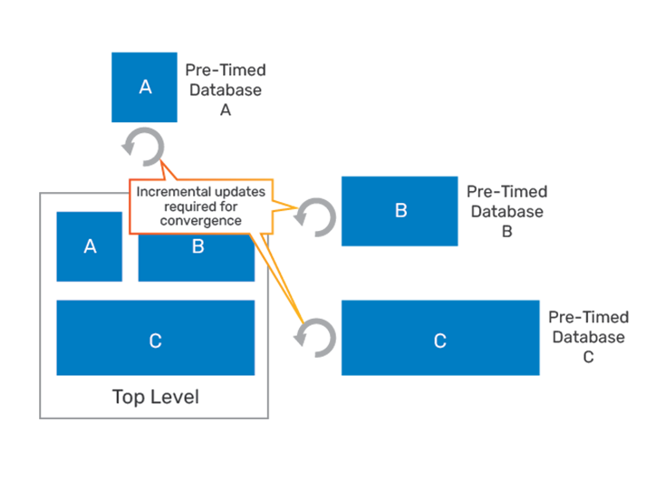
Though this solution reduces some of the capacity limitations of full flat analysis, it does come with several limitations.

The base-delay computation relies on having the correct loads at the outputs and slews at the inputs. By asserting arrival/ required times at the boundary pins of a block, and refining the assertions iteratively, some of the inaccuracies with other hierarchical approaches can be addressed. However, the CPPR adjustments needed for accurate path analysis cannot be addressed in this fashion. The CPPR adjustment depends critically on knowing the precise clock tags at the launch and capture clocks. If the clock tree is substantially outside the block boundary, such that the re-convergence points are outside the block, then accurate CPPR adjustment might not be possible.

Clock analysis has similar issues: if a clock buffer drives multiple blocks that are analyzed independently, the downstream information necessary to determine the propagation of clock and data phases through the buffer (e.g., for inferred clockgating checks) cannot be accurately determined in each block, leading to inaccurate path reports.

SI delay relies on having accurate timing windows available for all aggressor nets. Some iterative mechanisms can be employed to synchronize timing windows, if the coupling is across partitions. However, the clock-phase information associated with a timing window for a net that is outside a block might not be interpreted correctly, if the clock-phase is not present in the block.

Precise application of constraints for nets and paths that cross a block boundary also pose a challenge. For example, the user might wish to propagate constants through sequential elements. In this case, the constant propagation cannot be performed by simply asserting constants at block boundaries and then propagating them through the block. If multiple iterations of block analysis are required, the convergence is difficult to determine. In general, if the user’s constraints refer to the flat design context, the hierarchical approach must create block-level constraints from them, and then attempt to manage the block-level constraints transparently. Any incremental addition/updating of user constraints must be reconciled with the block-level constraint.

When one looks at signoff timing analysis, it is inferred that the results must be signoff accurate. Accuracy is the reason there is a whole market segment of tools dedicated to signoff timing. With this in mind, full flat analysis is the standard for handling all physical and electrical context-based impacts on timing analysis. The introduction of full flat distributed timing analysis in the Cadence Tempus Timing Signoff Solution has dramatically improved runtime and capacity. There is almost no limit to the design sizes that can now be analyzed flat. However, it is common for subsets of the design to go through final iterations just before tapeout. For these situations today, a full chip analysis is required in order to properly take into account the in-context effects or how a compromised solution such as an ETM or ILM approach can be used to save on the runtime of the entire design.

Einstein once said, “Everything should be made as simple as possible, but not simpler.” Applying this principle to the analysis of a block of a design means to time that portion flat because it is the most straightforward (i.e., “simple”) and accurate solution. Making the solution too simple results in the compromised solutions we have already discussed. So the question remains how to only time that portion of the design that is influenced by the changed block. The answer is scope-based analysis.

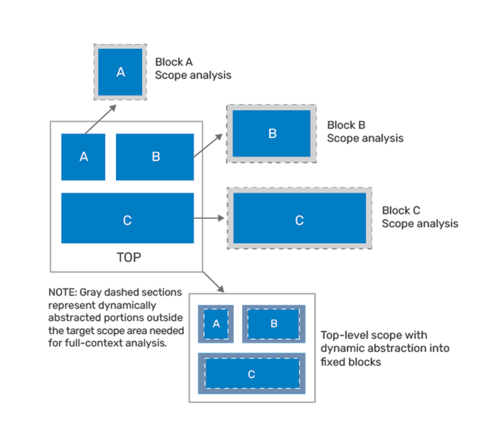
Cadence has developed, within the Tempus solution, the ability to dynamically abstract only those portions of the design that a user wants to analyze, and do it with full chip-level context. In this approach, users define the change space at the level of granularity equal to physical/logical block boundaries. Once the blocks or top-level scope is provided to the Tempus solution, dynamic abstraction of the design is done under the hood. The resulting carved out design is then analyzed which results in significant runtime and memory footprint reduction. Figure 5 shows pictorially that scope-based analysis can be run for blocks or the top level if that is the only portion of the design that was changed.

The timing closure and signoff solutions in use today have been extended to include advanced, more complex functionality to address SI and MMMC analysis and variation. Though these solutions extend capacity and reduce runtime, they are all compromised solutions for final signoff. Ultimately, the heart of a full timing signoff solution is still rooted in its ability to accurately take into account full chip-level design context. The only way to achieve this without compromising accuracy or physical design methodology is with full flat-level timing analysis.

Cadence has introduced the next generation of timing analysis tools in the Tempus Timing Signoff Solution. The Tempus solution both extends capacity and addresses runtime by scaling the use of distributed processing power with design size. Taking this one step further, the Tempus solution now introduces the concept of scope-based analysis to accurately and efficiently analyze portions of the design that have changed or are affected by the design change. At the root of the solution is intelligent abstraction of the affected design space, which is ultimately run in a true flat-level analysis. This solution comes without many of the compromises that are seen by utilizing ETMs or ILMs to maximize runtime and capacity. Nor does scope-based analysis require the iterative analysis and constraint refinement seen in existing alternative flows.

With the ability to run 100s of millions of cells with full flat analysis or intelligently run only a portion of the design at a fraction of the time, Cadence continues to introduce solutions that keep customers ahead of the design problems of the future.

Tempus Timing Signoff Solution