Addressing Process Variation and Reducing Timing Pessimism at 16nm and Below

If you’re like most design engineers, you’re getting your library files from your foundry or IP provider. This approach is fine in a number of scenarios: your design is at a larger process node, such as 90nm or larger; your design doesn’t require high speeds or performance; and/or your design is operating either at or higher than 3X the transistor threshold voltage. At larger nodes, timing margins simply aren’t a significant portion of overall timing constraints. But relying on these library files becomes problematic if you’ve got a highspeed or high-performance design and, particularly, if you’re designing at advanced nodes.

When foundries and IP providers create libraries for standard cells, I/Os, memories, and/or mixed-signal blocks, most of them perform simulations to model timing delays and constraints and add margins to cover timing variation. However, pre-packaged models from an IP provider or memory compiler may lack the accuracy needed, particularly since the exact context of the macro won’t be known until it is placed on the chip.

Process variation, which increases at advanced nodes, results in additional timing margins added to the libraries. This creates a tradeoff at smaller processes—either your design has to run slower so that you can have higher yield, or you lose some of your yield for a higher speed design.

IoT, wearables, and mobile applications are developed on advanced nodes to take advantage of the low-power and high-performance benefits of these processes. In order to ensure that you can take full advantage of the power, performance, and area (PPA) benefits of advanced processes, it’s critical to keep timing margins in check and to accelerate timing signoff by reducing timing margins.

Advanced-node design calls for many more library views to achieve high-quality silicon and also to avoid silicon respins resulting from inaccurate signoff analysis. It’s not uncommon at these processes to have low-, nominal-, and high-threshold cells, each with different power and performance characteristics, to manage leakage power. You’ll also find that it’s critical to characterize each library process corner over many voltages and temperatures, in order to accurately model instance-specific voltage variation or temperature gradients. For many advanced processes, alternative cell libraries are commonly offered to improve yield, trading off area and performance.

There are also now more contributors to timing variation to consider. For example, at advanced nodes, as gate length decreases, the single transistor threshold voltage (V_th) variation increases. At the same time, to preserve the low power and long battery life desired by applications such as IoT and wearables, the value of supply voltage (V_dd) goes down. As a result of these two scenarios, timing variation increases and becomes more pronounced. So, it’s no longer enough to run timing analysis on a slow process corner and a fast corner of a batch of wafers to determine whether a chip has met its timing constraints. Now there are significant variations across individual wafers and even at the intra-die level¹.

True, there are costs associated with creating entirely new timing variation models under a new methodology. But you really can’t afford to place extra timing margin on your cells. You need more accurate library characterization and variation modeling to reduce timing pessimism. The benefits of this will outweigh the initial investment.

There has been an evolution of approaches in static timing analysis (STA) to address OCV. Monte Carlo simulation is the most accurate in addressing timing variation, accounting for each timing arc, rising and falling edges or transitions, conditions for side inputs, and dependency on input slews and output loads. However, considering the number of cells in a library, the number of corners you’d need to simulate, and the number of slew/load multipliers in each cell, you’ll end up having to perform billions of such simulations for each library.

OCV derating was introduced as a first-order approach. With this process, you essentially attribute a single derating factor to all of your cell instances. The drawback is, depending on the length of the path you’ve chosen, your results will either be very optimistic or very pessimistic. Again, if your design is not a high-speed one, you might be able to live with these inaccuracies. But for high-speed designs like application processors, you’ll want more precision to reduce margins and improve design performance.

In the early 2000s, statistical STA (SSTA) emerged as a promising alternative approach to address OCV inaccuracies, delivering a complete statistical distribution. While highly accurate, it is expensive to create the SSTA libraries, and running the analysis requires a lot of memory and long runtimes. Plus, the timing signoff tools at the time were not ready for the amount of data being delivered.

Advanced OCV (AOCV) addresses path-length dependency to reduce pessimism. Essentially, you take each cell in your library, place it in a chain of the same cell, assume some parasitic elements in between, and come up with some timing derating factors as a function of chain length, early or late arrival, or rising edge or falling edge.

This AOCV methodology doesn’t account for whether the cell has multiple arcs from input to output and uses one arc, often the worst-case arc, to represent the derating factor. AOCV also doesn’t account for load on the output of the cell, input slew, or operating conditions for side inputs. The AOCV methodology assumes the chain will account for the load. But in a cell used in a real design, you can possibly find chains of buffers and inverters in the clock tree, but you don’t see chains of AND, OR, or other logic gates. So the AOCV model might be fine for some of your clock buffers and inverters, but nothing else. Further, since AOCV assumes similar statistical variability between instances of the same cell regardless of slew and load, it can still be either very optimistic or very pessimistic when compared to SSTA².

Statistical OCV (SOCV) models a more complete statistical representation as it accounts for pin-to-related pin dependency, the value of other side pins of the same cell, input slew, and output load, and provides sigma factors for early and late portions of the statistical distribution if they’re different. SOCV variation models enable near SSTA accuracy but without the expense of SSTA.

Finally, the Liberty Technical Advisory Board (LTAB) has converged on a unified Liberty Variance Format (LVF) that includes OCV modeling along with existing timing, noise, and power models³. Similar to SOCV, LVF represents variation data as a slew-/load-dependent table of sigmas per timing arc (pin, related_pin, when condition). Tables are supported for delay, transition, and constraint variation modeling. Major foundries are now working to support LVF at advanced nodes, and timing signoff tools have been updated.

Timing signoff tools, with the increased variation modeling fidelity of the SOCV/LVF model, use an SSTA engine to propagate statistical arrival time. Timing data values are represented concurrently by the statistical mean and sigma values. Users can always retrieve discrete representations of timing data and also report statistical and/or discrete representations as needed.

So how can we effectively create variation models for a given cell? For a given arc in a particular cell, we need to first determine which transistors will contribute to variation and which will not, and find a way to assess the impact on timing variation. We also need to consider the impact of input slew and output load, as well as the impact of all process variation parameters that need to be evaluated. As different transistors in the path behave differently, we create a delay variation surface for the impact that each transistor has on timing. If we combine these surfaces and they are fully correlated, we’ll end up with pessimistic results. How can we efficiently combine and create an aggregate standard deviation surface for all transistors in the cell, in order to have more accurate and less pessimistic results?

To model random variation, some considerations:

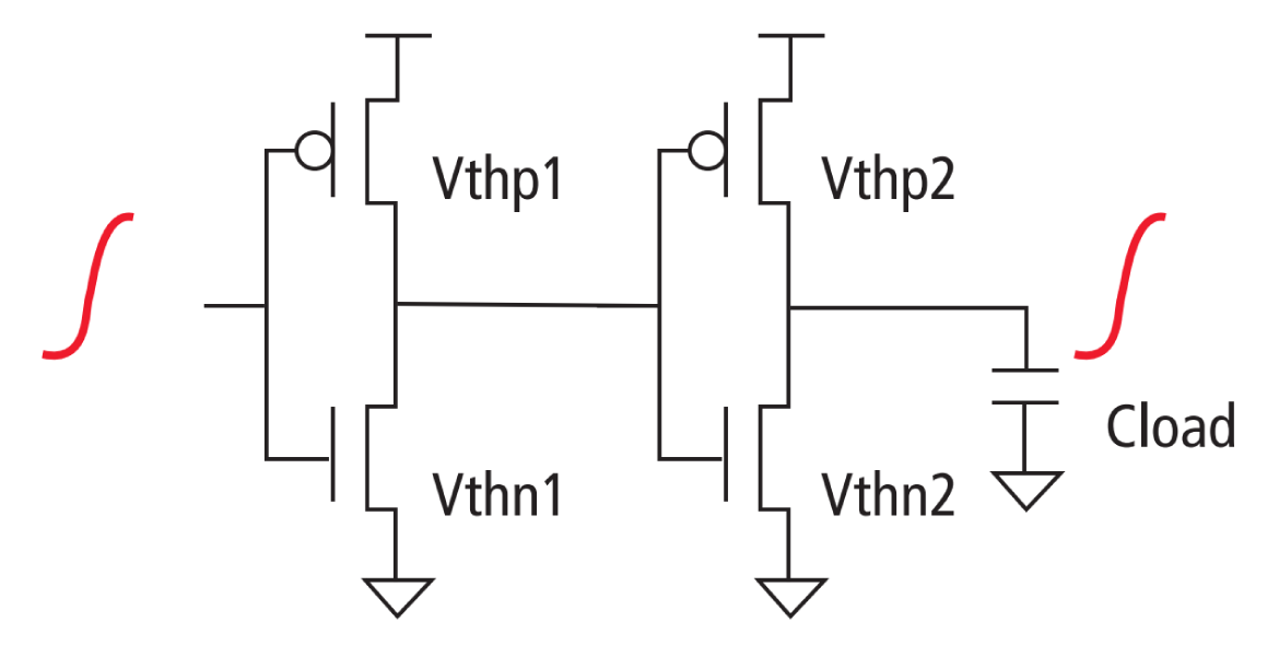
Table 1 shows random Vth variation for a buffer measuring rise-rise delay.

To provide the accuracy and speed that are so critical, a library characterization and variation modeling tool that creates LVF should be able to recognize different cells automatically and identify the stimulus that would result in worst-case conditions. Further, for a given cell and architecture, the tool should identify which transistors are contributing to variation and which ones are not.

Cadence offers a comprehensive Liberty library characterization suite for nominal characterization, statistical characterization and variation modeling, and library validation for standard cells, I/Os, memories, and mixedsignal blocks. The variation modeling tool results are tightly correlated in terms of accuracy to reference Monte Carlo simulations, but the tools run orders of magnitude faster. The accuracy as well as high throughput can be attributed to the tools’ patented Inside View technology for generating and optimizing characterization stimulus and the parallel processing capability that taps into enterprise-wide compute resources.

The statistical characterization and variation modeling technology offers some other advantages, too. Logic cone sensitivity analysis to identify which transistors are contributing to variation improves performance by keeping simulation size relatively constant, especially for multi-bit flops. Path delta constraint sensitivity removes sensitivity to cases where bisection has multiple solutions. With faster support of non-linear variation, the technology improves accuracy due to non-symmetrical variation.

The Cadence Liberate Characterization Portfolio consists of:

All tools in the Liberate Characterization Portfolio share a common infrastructure, fostering characterization productivity. Integration of these tools with the Cadence Spectre Accelerated Parallel Simulator (APS), which performs the simulation tasks “under the hood,” results in a 3X improvement in throughput compared to using a command-line use model. (External circuit simulators can also be used.) Output libraries are also validated with the Cadence Tempus Timing Signoff Solution, which supports OCV, AOCV, and SOCV/LVF technologies for faster, more accurate timing signoff. Because the statistical mean and sigma values are captured, the timing tool can propagate both values along the timing path; final timing reports provide both values for a more precise level of confidence. In addition, SOCV/LVF-based optimizations in the Cadence Innovus Implementation System result in improved density and reduced pessimism, compared to AOCV.

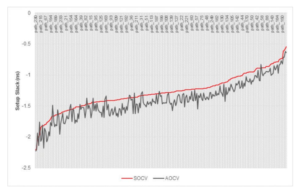
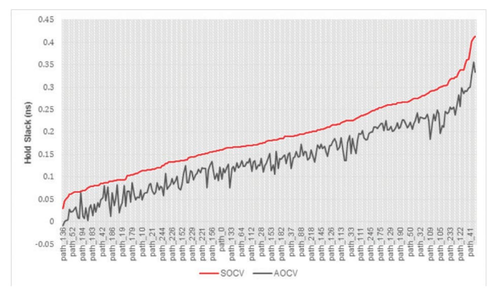
Figure 2 and Figure 3 show plots comparing setup slack and hold slack for the top 200 paths of a block running at a 1GHz clock frequency. When using a path-based SOCV/LVF timing signoff methodology rather than a graphbased AOCV timing signoff methodology, you can observe an average improvement of 150ps for setup slack and 200ps for hold slack.

At advanced nodes, creating and maintaining all of the library views needed can become a big design-flow bottleneck. Library characterization technology using an SOCV/LVF approach can help reduce timing pessimism and address process variation that is increasing significantly at smaller processes. With its Liberate Characterization Portfolio, Cadence is the trusted leader in library characterization technologies. Integrated with Cadence simulation tools and validated with digital implementation tools, the suite gives you the characterization accuracy you need to manage OCV at 16nm and beyond.

¹ Guide: “On-chip variation (OCV)”

² Article: “Signoff Summit: An Update on OCV, AOCV, SOCV, and Statistical Timing,” Industry Insights by Richard Goering, November 25, 2013

³ Article: “Liberty changes bring together nanometer OCV techniques” by Chris Edwards, Tech Design Forum, October 1, 2014