- Introduction
- Design Overview
- Step 1: Designing the System in AWR VSS Software
- Step 2: Creating the PCB/LTCC Within AWR Microwave Office Software
- Step 3: Designing the Antenna in AntSyn Software
- Step 4: Importing the MMIC for the PA and LNA
- Step 5: Designing and Simulating the Signal Path
- Step 6: Completing the Circuit
- Step 7: Importing the LNA for the Receiver
- Step 8: Completing the Module
- Step 9: EM Optimizing the Antenna Matching Circuit
- Step 10: Verifying System-Level Performance
- Conclusion
Application Note
LTCC Transmit/Receive X-Band Module with a Phased Array Antenna
Overview
Introduction
The X-band frequency range is widely used for satellite communications (SATCOM) because it provides a number of advantages over lower frequency systems, including resilience to interference and weather, smaller terminal size, higher data rates, and ability to provide remote coverage. SATCOMS are further enhanced through the use of active phased array antennas, which are made possible by advances in electronic packaging technology and semiconductor device performance. By employing space-saving, high-functionality system-on-chip (SoC), system-in-package (SiP), and low-temperature co-fired ceramic (LTCC)-based modules, SATCOM systems with active phased arrays offer greater flexibility and robustness.
This “how to” application note describes the steps to design a transmit/receive (TX/RX) module with a 2x2 phased array antenna (Figure 1) operating in the 8-12GHz frequency range. It highlights several innovative capabilities within the Cadence AWR Design Environment platform, including multi-technology and circuit/system co-simulation, as well as phased array modeling.
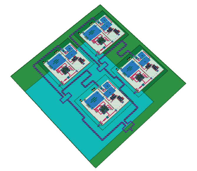
Figure 1: TX/RX module with 2x2 phased array antenna
Design Overview
This design example starts by highlighting the use of system-level characterization and RF circuit-design software for schematic entry and layout, then dives into electromagnetic (EM) simulation of the interconnects and bond-wire transitions. It continues by looking at each antenna as excited by a separate module composed of a PCB as the motherboard LTCC technology for embedded passive components and as a platform for the microwave monolithic integrated circuit (MMIC) and dies, a MMIC for the power amplifier (PA), a PA driver, a phase shifter, an attenuator, vendor or internally designed components, transitions such as bondwires, microstrips, and striplines (MLIN/SLIN) (Figure 2), and an antenna.
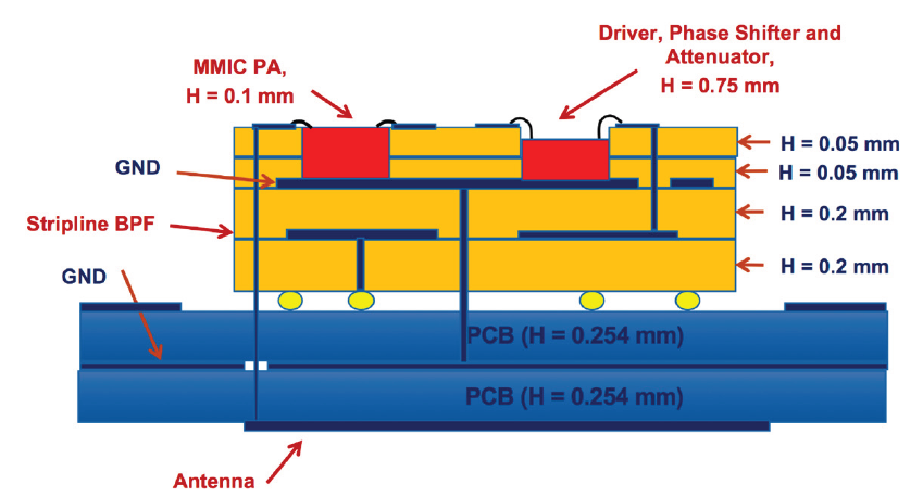
Figure 2: Simplified STACKUP for the module
Several Cadence AWR software tools are highlighted throughout the design flow, including AWR Visual System Simulator (VSS) software for system-level characterization, AWR Microwave Office circuit design software for schematic entry and layout, AWR AXIEM and AWR Analyst simulators for EM simulation of the interconnects and transitions (bondwires), and AWR AntSyn antenna synthesis and optimization software for the phased array antenna design, as well as several specialized synthesis wizards.
Step 1: Designing the System in AWR VSS Software
Figure 3 shows the system design diagram for this example, which uses the AWR VSS TX/RX-mode testbench. At the system level, hierarchy was used to inject signals on the left (TX continuous wave [CW] test) and on the right (RX CW test), which could be switched with AWR VSS components (middle). The TX/RX module was used as a subcircuit within the system design.
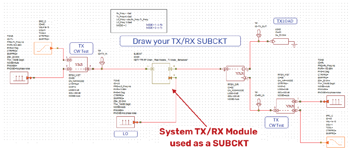
Figure 3: System design diagram, including TX/RX module subcircuit
Figure 4 highlights the TX/RX module subcircuit, which was modeled in the AWR VSS software with behavioral models. Inside the subcircuit are the switches, filters, and amplifiers; the mixers and other components are shown outside the model.
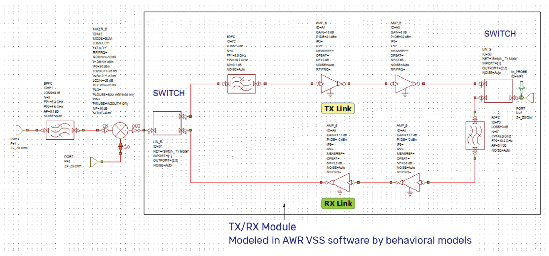
Figure 4: Detail of the TX/RX module subcircuit
After building the system design, the RF budget (RFB) utility within the AWR VSS software was used to make RF cascaded measurements such as gain, noise figure, and third-order intercept. The RF inspector (RFI) frequency-domain utility in the AWR VSS software was then used for spurious analysis of the TX mode and RX mode (Figure 5) of the module.
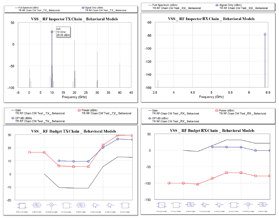
Figure 5: RF cascaded measurements and spurious analysis of the TX mode and RX mode
Step 2: Creating the PCB/LTCC Within AWR Microwave Office Software
Next, the PCB and LTCC were designed. The PCB contains two dielectric layers, on top of which sits an LTCC, including a MMIC PA. The process creator technology in the AWR Design Environment software generated the STACKUP and intelligent net (iNet) technology was used for generating the layout files, cells, and other substrate blocks.
The process design kit (PDK) of the LTCC can be set as a standalone, as can the PCB (Figure 6). Creating both at the same time enables designers to save time by using the multi-technology feature with the software. Once the STACKUP was created (Figure 7), it was an easy process at any point to draw the layout of either the PCB or LTCC, or a combination of both.
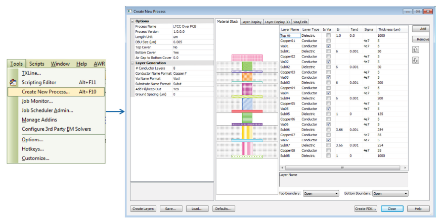
Figure 6: Process creator tool
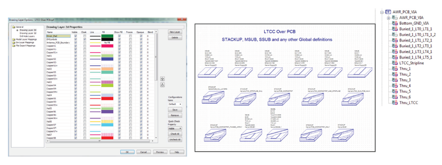
Figure 7: The process creator generates global definitions, a layout process file, and via layout cells
Step 3: Designing the Antenna in AntSyn Software
The next stage was to design the antennas. The 2x2 array was designed using the AntSyn EM-based antenna synthesis tool. The goals of the antenna design and classes of antennas to explore were specified and then the AntSyn tool found the optimal antenna automatically based on the chosen parameters.
The 2x2 patch antenna array was set to 10GHz and several parameters were also specified, including return loss and gain. The resulting optimal antenna design model from AntSyn software was then exported directly to the AWR AXIEM planar EM simulator (Figure 8).
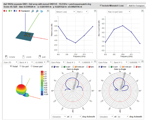
Figure 8: The AntSyn antenna model for export to the AWR AXIEM simulator
Once imported into the AWR Microwave Office software specifically for EM simulation within the AWR AXIEM module, the metal layers were mapped and the simulation run. As Figure 9 shows, a good match was reached.
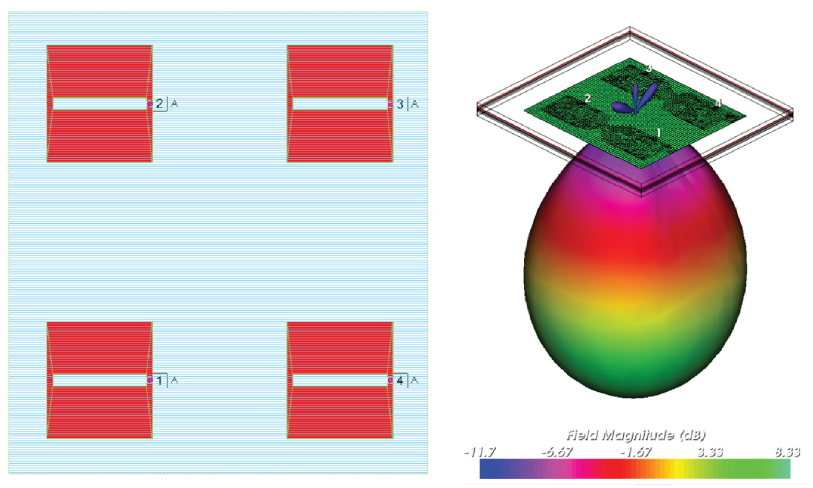
Figure 9: AWR AXIEM simulation results
Step 4: Importing the MMIC for the PA and LNA
The AWR Design Environment software supports the use of multi-technology, which allows designers to include several PDK technologies such as PCBs, LTCCs, MMICs, and RFICs in the same project. The MMIC was imported with all the MMIC process definitions, including global definitions, low-pass filter (LPF), schematic, layout, linear and nonlinear models, and more (Figure 10).
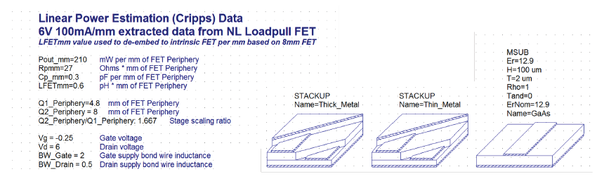
Figure 10: The MMIC was imported with all the process definitions
Wiring the MMIC PA
Once the MMIC PA was imported, it was placed in the layout and the iNets tool was used to add the bondwires, vias, and bias lines (Figure 11).
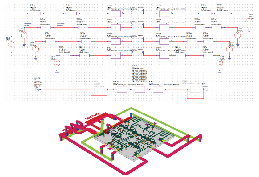
Figure 11: The iNets tool was used to add the bondwires, vias, and bias lines
Step 5: Designing and Simulating the Signal Path
Next, the Analyst software was used to design and simulate the signal path, with transitions from the MMIC PDK to the LTCC PDK using dual bondwires. Because it is a 3D EM simulator, the Analyst software can work with multiple technologies, which, in this example, includes a gallium arsenide (GaAs) MMIC pad, an LTCC pad, and a bondwire model. The distance between the bondwires and their length was optimized and the transitions were optimized up to 50GHz.
Using External Library Parts
Instead of designing a MMIC from scratch, external library parts were imported into the model, including a PA driver, a phase shifter, and an attenuator. The cell was generated, named, and then imported. This was easily done in a schematic that is synchronized with the layout (Figure 12).
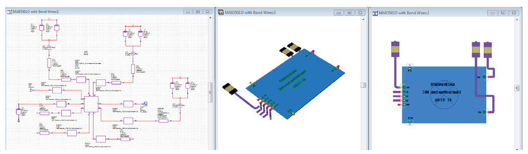
Figure 12: External library parts were imported into the model; the schematic was synchronized with the layout
Designing the Filter
The Cadence AWR iFilter synthesis wizard was used to design a stripline bandpass filter (BPF) using the iFilter interdigital option (Figure 13). The filter was imported into the model, optimized in the AWR Microwave Office software, and directly EM simulated and optimized using the AWR AXIEM EM simulator (Figure 14). Once optimized, it was then re-embedded in the model.
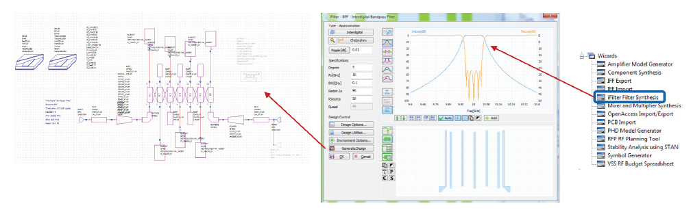
Figure 13: The iFilter interdigital option was used to design a stripline BPF
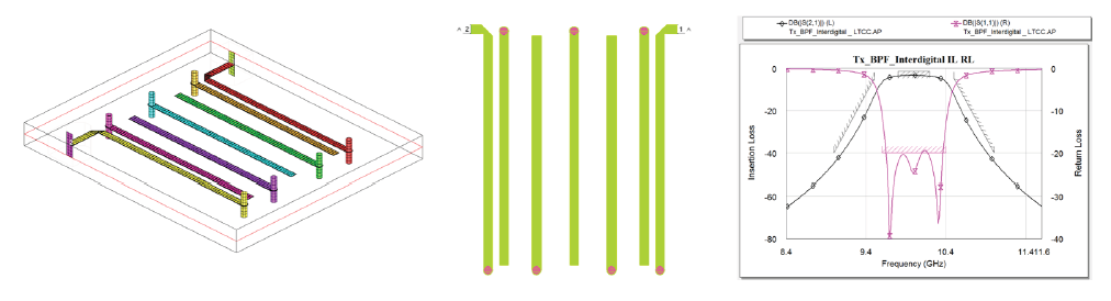
Figure 14: The filter was simulated and optimized directly in the AWR AXIEM simulator
Step 6: Completing the Circuit
With the designs finished, everything was then combined into a single schematic, which included the stripline BPF, the vendor models, the imported MMIC PA, and all of the transition models. Figure 15 shows the schematic layer in both the 2D and 3D views.
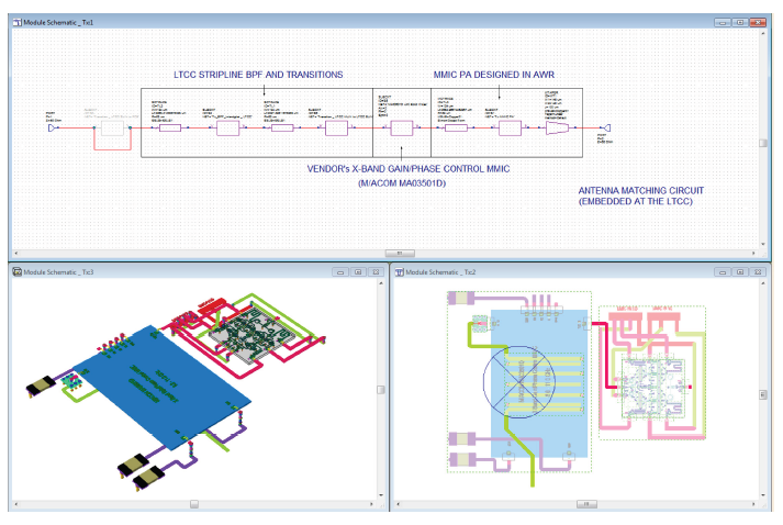
Figure 15: 2D and 3D views of the schematic of the entire circuit design
Transitioning the LTCC MicroStrip to the Stripline
The AWR AXIEM software was used to simulate and optimize the transition of the LTCC microstrip to the stripline (Figure 16). This is another example of how the transitions can be designed inside the AWR AXIEM EM simulator for an optimum transition up to 40-50GHz or higher.
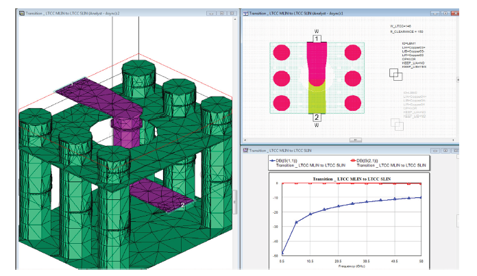
Figure 16: The transition of the LTCC microstrip to the stripline using AWR AXIEM software for simulation and optimization
Step 7: Importing the LNA for the Receiver
As with the MMIC PA, the LNA model was imported from another project and bondwires and bias lines are added. In Figure 17 the schematic, layout, and 3D layout have been combined into the model.
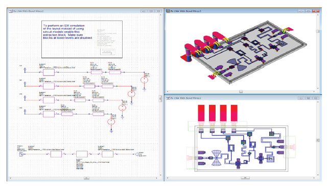
Figure 17: The schematic, layout, and 3D layout have been combined into the model
Importing Parts for the Receiver
Next, the parts for the receiver were imported, including an attenuator and a phase shifter (Figure 18).
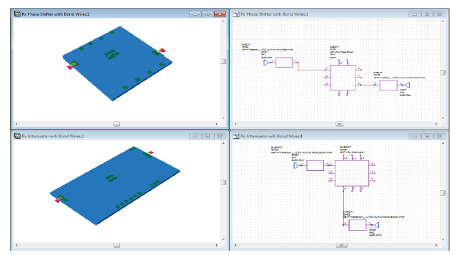
Figure 18: An attenuator and phase shifter were imported into the model
Integrating the RX Chain
Integration of the RX chain was carried out in the circuit schematic (Figure 19).
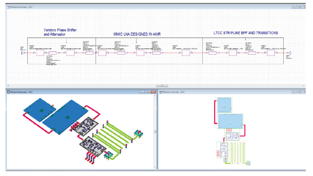
Figure 19: Integration of the RX chain
Step 8: Completing the Module
The TX/RX module in this example used a time-division duplex (TDD) approach. A vendor switch model was added (S3P and layout). Figure 20 shows the schematic model, layout model, and the transitions.
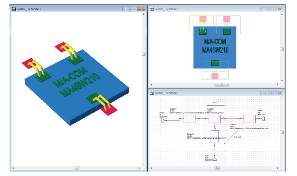
Figure 20: The schematic model, layout model, and transitions
Adding Vias
Once the model of the module was complete, the TX and RX designs were integrated and ground or via fences were added. The vias can be drawn either at the schematic or layout level. Figure 21 shows the schematic and the 2D and 3D views of the layout.
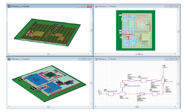
Figure 21: The schematic (lower right) and 2D and 3D views of the layout of the module with ground or via fences
Adding Passive Components
With the model complete, the entire 2x2 model could be designed. For that, the passive components synthesis wizard was used for the splitter. Figure 22 shows the wizard dialog box with a Wilkinson divider selected as the component type with a single section, centered at 10GHz.
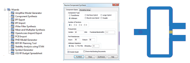
Figure 22: Components synthesis wizard dialog box
Step 9: EM Optimizing the Antenna Matching Circuit
The matching of the antenna was then performed, which was a bidirectional matching from the antenna into the PA itself. The AWR Microwave Office circuit elements can be used to parameterize the inductors/capacitors in the AWR AXIEM or Analyst simulators. For example, MRINDNB2 can be used for a rectangle inductor and MICAP for an interdigital capacitor. Many other models are available, and imported PDK elements can be used as well. Once the EM models were parameterized, the antenna matching circuit could be optimized. Figure 23 shows the EM optimization for the antenna matching output impedances (top right) of the PA.
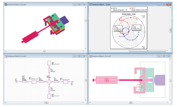
Figure 23: Once the EM models were parameterized, the antenna matching circuit could be optimized; EM optimization for the antenna matching output impedances is shown in the top right image
Figure 24 is the schematic view of the complete module showing the 2x2 model structure with the antenna and the 2D view of the layout structure with the antenna.
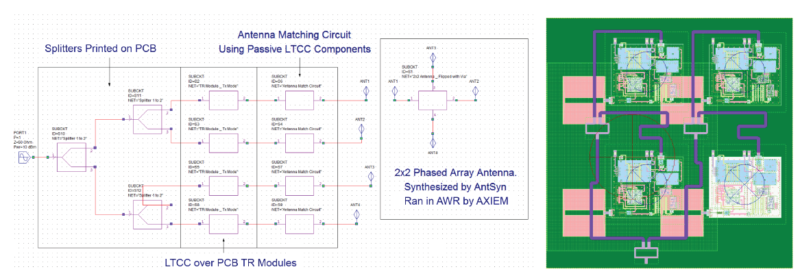
Figure 24: Schematic view of the complete module and 2D view of the layout structure with antenna
Coupling the Antenna and Circuit Simulations
Any antenna designed in the AWR AXIEM or Analyst EM software is excited by some circuit, which has an effect on the radiation. As the antenna scans, the input loads change, which affects the PA loads and performance. The in-situ measurement capability in the AWR Microwave Office software accounts for coupling.
The blue line in the antenna plot on the right in Figure 25 is the effects of the antenna when the model is connected and the black line within is the standalone without the effects of the model. The software gives designers a major advantage by enabling them to see the radiation pattern both with and without the circuit.
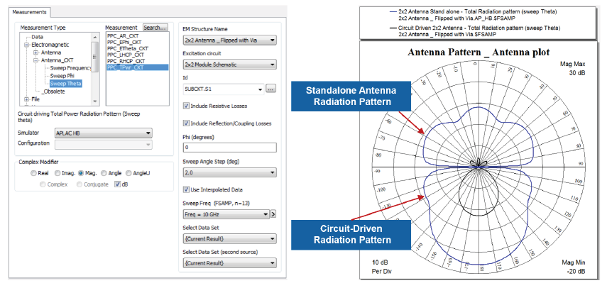
Figure 25: Radiation pattern, with and without the circuit
Figure 26 is a 3D view of the standalone and circuit-driven antenna radiation pattern. The pattern with the circuit is on the right and the pattern without the circuit is on the left.
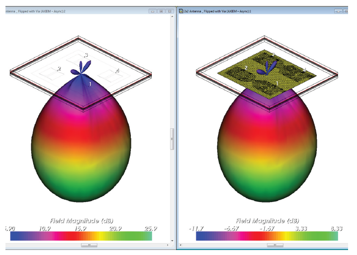
Figure 26: 3D view of the standalone (left) and circuit-driven (right) antenna radiation pattern
Step 10: Verifying System-Level Performance
The final step was to verify the performance of the module at the system level using real signals. The model was imported into the AWR VSS software and modulated signals such as quadrature phase-shift keying (QPSK), quadrature amplitude modulation (QAM), wireless local area network (WLAN) 802.11, LTE, 5G, and others, were injected into the module for testing. Figure 27 shows the error-vector magnitude (EVM) (top left), the spectrum (top middle), the modulation (top right), the spectrum (lower left), and the spectrum of the single tone (lower right). The lower middle is the entire design.
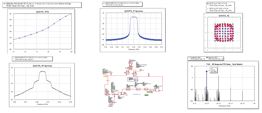
Figure 27: Performance system simulations of the module
Conclusion
The AWR Microwave Office circuit design software, AWR VSS system design software, and AntSyn automated antenna synthesis were used to design an integrated 2x2 TX/RX module and phased array antenna. The multi-technology capability in the AWR Design Environment platform enabled the designer to use different technologies, including gallium arsenide (GaAs) chips, LTCC modules, and Duroid boards, seamlessly at the circuit, layout, and EM simulation levels, all within the same project. AWR software co-simulation provided the ability to work at both the circuit level and system level in a single environment. The software’s specialized synthesis tools were useful for designing the filters and components. EM simulation was easily used where needed without leaving the AWR Microwave Office environment.